PROBABILITY and EXPECTED VALUE

We begin with three definitions of probability.

CLASSICAL: the probability of an event is the ratio of the number of ways an event can occur to the total number of outcomes when each outcome is equally likely. An EVENT is the outcome of an experiment.

let s = # of ways of getting A

f = # of ways A cannot occur

If we define success as picking an ace from a deck then

RELATIVE FREQUENCY:  let n be the number of successes, i.e., the occurrence of A, and let m be the number of trials
As the ratio of n to m approaches the probability of the event A:

i.e.,

SUBJECTIVE: Degree of rational belief.  The probability of an event occurring is what you feel it to be. This is closely akin to the notion of a prior probability in Bayesian analysis.

SOME MORE DEFINITIONS
Consider an experiment with N possible outcomes. The set of outcomes in called the sample space.
An event is a subset of the sample space, call the event A.

The probability of an event "A" is the number of outcomes in "A" divided by the number of elements in the sample space.

Example: Flip two coins. The possible outcomes are

{HH, HT, TH, TT} = sample space

Example: Choose a card at random from a fair deck. What is the probability of a face card or a heart?

A = face or heart

there are 13 hearts and 12 face cards, but 3 of the hearts are face cards

SET THEORY

The (set or event) C consists of the set of all points x such that x lies between zero and infinity.

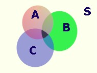
The set C consists of all points x such that x is in both A and B.

This is an example of the null set.

COMPLEMENT OF AN EVENT

The complement of an event A is denoted by .

Let S be the sample space, of which A is a subset i.e., then the complement of A is the set of points left after we take those belonging to A out of the sample space S.

Using a Venn diagram

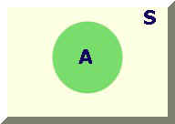
is the yellow shaded portion.

Using set notation

Example:

MUTUALLY EXCLUSIVE EVENTS

If A and B are mutually exclusive events then the occurrence of one precludes the occurrence of the other.

Examples:

1. on a coin flip H and T are mutually exclusive

2. on the roll of a die the events "roll a 1" and "roll a 3" are mutually exclusive.

MUTUALLY EXCLUSIVE AND COLLECTIVELY EXHAUSTIVE

If A and B are mutually exclusive they cannot both occur at the same time. If they are collectively exhaustive then they contain, between them, all possible outcomes in the sample space.

Example:

1. On a coin flip H and T are mutually exclusive and collectively exhaustive.

2. "Roll a 1" and "Roll a 3" are mutually exclusive but not collectively exhaustive.

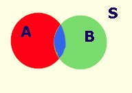
INTERSECTION

Let X represent the points of a sample space S.

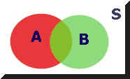
Let A and B represent two subsets of this sample space

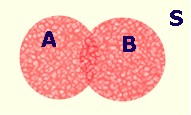
We can represent their intersection algebraically as shown at the left. In the diagram the intersection is the lens formed where A and B overlap.

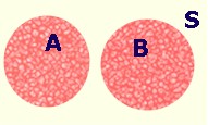
Suppose A and B do not have any points in common, i.e., they are mutually exclusive, then the Venn diagram representation looks like:

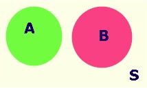If a point belongs to A then it cannot belong to B, and vice versa.   There are no points in common to both A and B.

We can extend the idea of intersection to more than two sets.

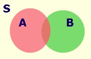
UNION OF TWO EVENTS

The set of points that are in either or both of two events

These two Venn diagrams differ to the extent that there are no points in common between A and B in the second diagram.

COMPLEMENTARITY AND CONDITIONAL PROBABILITY

COMPLEMENTS

Let the sample space contain N sample points and event A contain "a" of these points. Then from our previous definition

consists of (N - a) points, so

Example: Define event A as rolling a single die and getting a one. As a result, we define as rolling a 2, 3, 4, 5 or 6

Now we are asked to find the probability of rolling a 2 or greater

CONDITIONAL PROBABILITY

Consider the type of question such that we are interested in the occurrence of one event given that another has occurred

In set notation

since we know B has occurred we need not worry about all of S


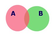
Our sample space is only the points in B and AB is the set of points common to both A and B, shown by the darker lens in the diagram.


Suppose that there are N points in the sample space, "b" points in B and "a" in the set A. Also, let there be W points in common between A and B.

The relative frequency of A|B can be determined from

and using our definition of probability

also

Example: Compute the probability of H on the second toss of fair coin given H on the first toss.

S = {H₁H₂, H₁T₂, T₁H₂, T₁T₂}

Example: Let A be the event 2 is drawn

B be the event Heart is drawn

Note that in both of these examples the two events are independent. What test for independence can you devise from this result?

MULTIPLICATION RULE

There are W points in the blue lens, a in the set A, and N in the sample space. From this we can calculate the probability of the intersection.

INDEPENDENCE

If A and B are independent then the fact that one has occurred has no bearing on whether or not the other occurs.

Example:

The first flip of the coin has no bearing on the outcome of the second flip.

Example: let A be the event a 2 is drawn

let B be the event a Heart is drawn

P(B) = 1/4

P(A) = 1/13

There is a special multiplication rule for independent events.

ADDITION RULE

Note that we have to subtract out the points in common, otherwise we would double count.

Example: Choose a card at random

A = face card

B = heart

Suppose two events are mutually exclusive, i.e.,

then

Since sets A and B don't overlap we don't have to subtract for double counting.

Question: Can two events be both mutually exclusive and independent?

but

An interactive notebook will help cement these notions.

BAYES RULE

Suppose we have the events A, B.

Upon rearranging 1 and 2,

equating these two gives

rearranging

Example: There are three chests in a room. Each chest has two drawers each containing a single coin

An individual staggers into the darkened room, opens a drawer, grabs a coin and staggers out. In the light it is observed that he has a gold coin. What is the probability that he got it from chest II?

A = gold coin

B = chest II

MARGINAL PROBABILITY

We can arrange much of our information into a table

The probabilities on the edges of the table are marginal probabilities.

RANDOM VARIABLES AND PROBABILITY FUNCTIONS

Definition: A random variable X is a function or rule that results in a mapping from the sample space to the real numbers:   X:S ==> R

or

A random variable takes a possible outcome and assigns a number to it.

Example: Flip a coin five times, let X be the number of heads in five tosses.

X = { 0, 1, 2, 3, 4, 5}

Definition: A probability distribution assigns probabilities to all possible outcomes of an experiment.

Example: The experiment is five flips of a coin, the random variable counts the number of heads and the probability distribution assigns a set of likelihoods to the possible outcomes.

If we were to do more examples we would surmise the following axioms of probability

Any probability must be between zero and one.  The sum of the probabilities assigned to all of the possible outcomes must be one. 

A third, less obvious axiom is

The probability of the union of all the disjoint sets must equal the sum of the probabilities of those sets occurring individually.

EXPECTATION

We are now prepared to introduce the notion of mathematical expectation. We begin the development with an example.

Example: Flip two coins. For each head that appears you receive $2 from your rich uncle. For each tail you pay him $1. The outcomes, or points in the sample space, of the experiment are

As an astute player you should be interested in the probability of a particular $ outcome of the game.  The game assigns a dollar value to each of the four possible H-T outcomes. Since two of them are monetarily the same we get the following random variable and distribution:

After explaining the above game, your uncle asks how much you are willing to pay in order to play.

You are not interested in your expected winnings on any given pair of throws, but you are interested in your long run winnings, or what you could expect to win if you played the game many times. We could repeat the experiment an infinite number of times and calculate the average payoff per trial. There is an easier way to determine this average than flipping coins for the rest of our lives.

Expected value is merely a weighted average.  Your grade point average is a weighted average. The weights in the coin toss game are the probabilities that an outcome will occur.

Think of how we would calculate the mean if we were to flip a large number of pairs of coins.

We would use the following:

Ex =

We read this as "The expected value of x is equal to the population mean; it is computed as the frequency weighted average of the values taken by the random variable x.

where x_i is our winning of the i^th type and f_i is the number of times that outcome occurred in N trials.

But note that f_i/N is nothing more than a probability when .

Since our probability distribution has already letit seems reasonable to use

for calculation of our expected winnings.

For the coin game

so

Our long run average winnings will be $1 per toss. We would never pay more than that to play.

If we wish to find the variance for our winnings we could again use expectations. Namely,

This is a definition. With time and space we could demonstrate its relationship to the population variance you may have learned about in your basic statistics course.

For the coin game

There are some general rules for mathematical expectation.

RULE 1

RULE 2

RULE 3

RULE 4

RULE 5

As a note: X, Y are random variables with a joint probability function.

Also,

but,