VI. SIMPLE REGRESSION

A. CRITERIA OF FITTING A LINE

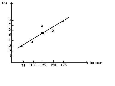
Suppose that we have observed some data on income and tea consumption

1

We wish to fit a straight line to this data. Clearly, it cannot pass through all the points. This leaves us with the problem of how to fit the line.

The equation for the line will be

whereis the point on the line that corresponds to a given x, contingent on our choice of a and b.

Let

be the difference between the fitted value and the observed value of the dependent variable.

a. One possible criteria for the selection of a best line is that line which makes the sum of the e_i as close to zero as possible

This has one obvious drawback

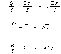
There are a large number of choices of a and b that will make Q/5 zero.

b. One way to cure this problem is to use

Analytically, this is very difficult and really is a problem in linear programming.

c. A final consideration is the sum of squared errors, i.e.

This puts very heavy emphasis on large errors, e_i and is analytically tractable.

However, before solving for estimates of the a and b we shall present a more formal statement of the problem.

B. MATHEMATICAL MODEL

We can show the relationship between tea consumption and income as a conditional probability density .

The problem is that we are not capable of observing a deterministic relationship between Y and X.

Reasons:

1. relationship is inherently stochastic

2. we observe X and Y only imperfectly

3. there is more to Y consumption than income X.

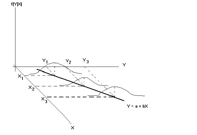
Instead, the situation appears as in the following diagram. For a given value of the independent variable there are many possible realizations of the dependent variable. When we collect sample data we observe only one possible such realization for a given value of the right hand side variable. The figure shows the expected value of Y conditional on X as the heavy line in the X,Y plane.

Generally, we often focus our attention onthe population regression function where

A convenient assumption is that the population regression function is linear in X.

The population regression is denoted

where u is the unobservable, true disturbance.

From the sample we find

are our estimates of a and b. is the observed error.

Before considering procedures for constructing estimators let us consider two properties of the population regression function.

PROPERTY 1

Proof:

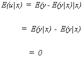
This property suggests that deviations from the population regression function have a mean of zero, given X.

PROPERTY 2

Proof:

Now

since

This property implies that the disturbance is uncorrelated with the independent variable.

Some assumptions:

1. a.

or

b.

2.

3. The X are constants in repeated samples of size n.

PROCEDURES FOR ESTIMATION

1. Analogy

We have the sample regression function

We wish the following to be true

1.

2.

These two items are the sample properties analogous to the two for the population that we just discussed. The first one says that on average the residuals should be zero. The second one says that the residuals should be orthogonal to the independent variable.

These two conditions can be written, upon substitution as

1.

2.

Carry the summation signs through

1.

2.

These can be further simplified

1.

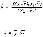
We now have two equations in two unknowns which can be solved to give

2. MINIMIZE THE SUM OF SQUARED ERRORS

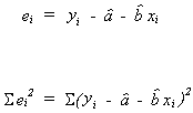
We can differentiate with respect toand get the first order conditions for a minimum. The two equations can then be solved for the appropriateand.

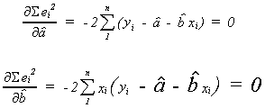
We recognize these two equations as the same as those in the previous procedure, so we are done.

3. MAXIMUM LIKELIHOOD

Consider a sample of independent and identically distributed r.v.'s, u_i, all having the density function. We can write the likelihood function as

Recall that we can state the principle of maximum likelihood estimation as:

Choose the estimator,, which maximizes the likelihood that the sample was generated by a probability distribution of the assumed type.

Assume then

and

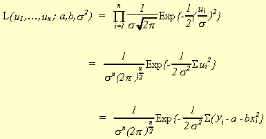
Maximizing L is accomplished by minimizing the exponent. Taking logs will simplify this task.

Now,

(1)

(2)

(3)

(1) and (2) are the "normal equations" that we have seen twice before.

We can solve (3) for an estimator of

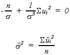
We have constructed maximum likelihood estimators of a, b andunder the assumption that the errors are normally distributed. Note that the denominator of the error variance estimator is scaled by n, not n-1.

Theshould be considered functions; rules for converting sample information into guesses about the population parameters. The rule is a random variable, until we plug in some sample information.

PROPERTIES OF OUR ESTIMATORS

1. EXPECTED VALUE

We will investigatefirst.

Define

We should note two things about

1.

2.

proof:

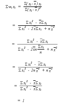
Using our definition of w_i

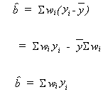
but

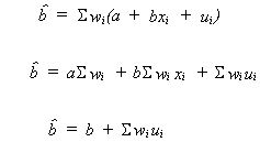
because of the two properties of w_i noted above

recall Eu_i = 0

is unbiased

Now consider

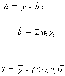
rearranging

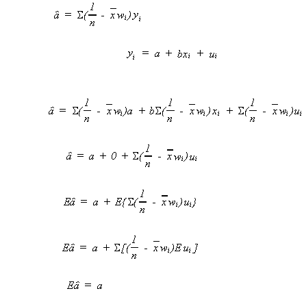
We will defer consideration of the bias of estimators foruntil a later date.

2. VARIANCES

Again we will considerfirst. By definition

Recall

so

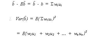
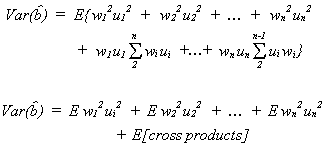
recall our assumptions

So

recall

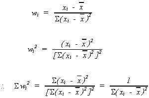
Finally,

From this expression for the variance of the estimator, we can see that our estimator is more precise, the greater the dispersion of the independent variable.

1

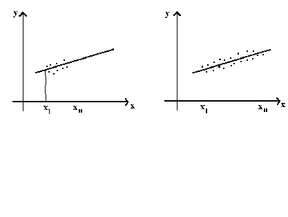
In the left panel we observe y for only a small range of x so there is some doubt as to the relationship between x and y as x becomes large. This doubt is measured by the variance of. Alternatively, if you must balance a beam on top of two points, are you more confident in the beam remaining balanced if the two points are close together or far apart?

The variance ofis easily found

recall

with the expectation all the cross products drop out so our concern is with

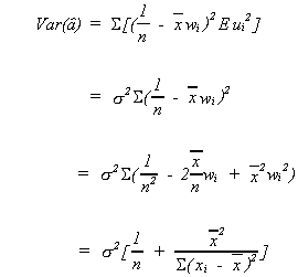
3. BEST LINEAR UNBIASED ESTIMATORS (BLUE)

Within the class of linear unbiased estimators ofandthere should be one that has the smallest variance.

By linear we mean the estimator is to be linear in Y. Unbiasedness is clear. By "best" we mean the estimator has the smallest variance of any estimators.

2

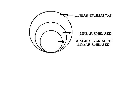
We have derived the OLS estimator and demonstrated that it is unbiased. But, in the class of linear unbiased estimators does it have minimum variance?

Let us construct an arbitrary linear estimate of b.

recall

In order for b^* to be unbiased the following must be true

We impose these restrictions so

The variance for b^* is

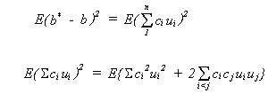
Taking expectations

so

So we wish to

s.t.

Set up the Lagrange expression

To find the constrained minimum we set the first order condition to zero

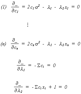
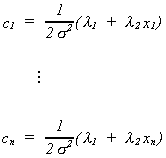
Solve (1) through (n) for the c_i

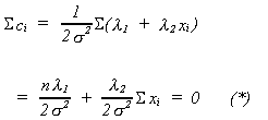
Recall, that is, observe the (n + 1)^th equation. So

Now multiply each of the c_i by x_i and add them up to obtain the (n + 2)^th equation

Solving (*) and (**) forandwe get

from (*)

substitute into (**)

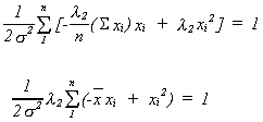
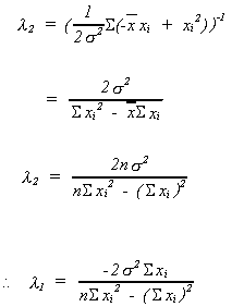
Substituting back into the first order conditions we get

OLS for b is BLUE.

CONSISTENCY

Recall

If

then the sequence of estimators is said to be consistent.

Our estimator is

with variance

since

recall

By Chebyshev's inequality

as, the denominator of the R.H.S. alsotherefore

AN UNBIASED ESTIMATOR FOR THE ERROR VARIANCE,

Recall

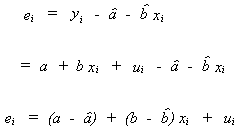
knowingandfrom above we can write

Note that the second and third terms represent two linear restrictions.

Let

it is our job to choose k so thatis unbiased.

Taking a closer look at the numerator. We cam rearrangeto get

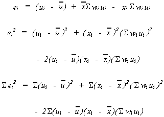
Now take expectations

Note 1:

Note 2:

Note 3:

Therefore

and

is an unbiased estimator for.

Note the following:

1. k = 2 corresponds to the number of linear restrictions on the u_i.

2. k = 2 corresponds to the number of parameters we have estimated in constructing the e_i.

3.

VI. F. HYPOTHESIS TESTING

Recollections

1.

2.

3. Ifandthen

Consequently,

define

and not that thein denominator and numerator cancel to get

EXAMPLE

Let y = GPA score

x = GRE score

Some date has been collected on these two variables. We wish to estimate the relationships

y = a + bx + u_i

n = 8

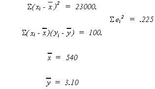
From the data

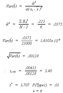
Therefore, we cannot reject the null hypothesis. Note that I chose critical value for a two-tail test.

REGRESSION WITH TWO INDEPENDENT VARIABLES

Specify the PRF as

or

Subscript of 1: variable number of dependent variable.

Subscript of 2: denotes variable x₂

Subscript of 3: denotes variable x₃

Subscripts to left of decimal are primary subscripts. The first is the dependent variable, the second indicates the variable to which theis attached.

The secondary subscript is to the right of the decimal indicates the other variables present in the model.

ASSUMPTIONS

1.

2.

3.

4.

5. There is not a setandsuch thatfor all i simultaneously.

INTERPRETATION

intercept

is change in y for a 1 unit change in x₂, holding x₃ constant

is change in y for a 1 unit change in x₃ holding x₂ constant

OLS estimators:

Again we wish to minimize the residual sum of squares (RSS)

Using the appropriate calculus we get the normal equations

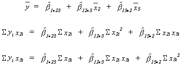
The intercept is obvious.

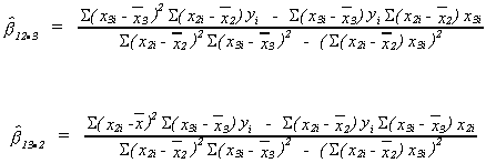
The three equations can be solved to yield the other two unknowns.

VARIANCES FOR SLOPE ESTIMATORS

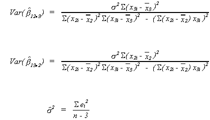
since we have used the n observations to calculate 3 parameters in constructing the numerator.

Note the following

1. since

2.

since in the simple case

COEFFICIENT OF DETERMINATION, OR THE GOODNESS OF FIT

R² shows the proportion of variation in the dependent variable that is explained by the independent variables.

We note the following

and define

or

AN EXAMPLE OF THE COEFFICIENT OF DETRMINATION AND THE COBB-DOUGLAS PRODUCTION FUNCTION

or

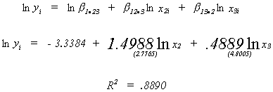
so ~ 89% of variation inis explained by our model.

COMPARING R² VALUES

Recall

Nowis a constant. As we throw in more variables, even if they are really garbage, will decline and so R² will go up.

It seems that we should correct R² to account for the indiscriminate addition of variables, i.e., a penalty. So

or

for the example

Constructing a model on the basis of a highis bad procedure. We should be concerned with logical and theoretical relevance of variables. Beyond that we should consider correct signs and significance of the estimates.

PARTIAL CORRELATION

Sometimes our interest may go beyond the simple goodness of fit measure. We may be interested in knowing the explanatory power of the jth variable once we have included the other j-1 variables. We begin with the simple correlation coefficient, which is closely related to the OLS slope coefficient in the simple regression model (can you derive the relationship?). Then we consider partial correlation.

Define the simple correlation coefficient as

we could calculate this for all pairs of variables in the model

1. -1 < r < 1

2. measure of linear association

3. does not imply cause and effect

Also, if there is more than one independent variable it does not reflect the true association between say x₂ and y.

That is, we would like to know the degree of linear association between x₂ and y controlling for x₃.

Define the following

so

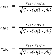
called first order correlation coefficients.

INTERPRETATION

1.

2. andneed not have same sign

3. may be interpreted as the proportion of y variation not explained by x₃.

HYPOTHESIS TESTING WITH TWO INDEPENDENT VARIABLES

our observed t is

which for 12 df is in the critical region for= .05 and a two tailed test.

CONFIDENCE INTERVAL

Let's build a 95% confidence interval for

Note that zero does not lie in this interval. So, at the .05100% significance level we can reject the hypothesis thatis zero.

FISHER'S F-TEST

We may wish to know if bothandare linearly related to Y. That is, we want to know if bothandare simultaneously zero.

Note that if

It is not necessarily true that the intersection of these two events has probability.

We wish to test at the

Doing a t-test on each will not produce the desired significance level.

Define the following terms

We can set up the following ANOVA table

Source of variation	Sum of squares	df
Due to Regression (ESS)		2
Due to Residual (RSS)		n-3
TOTAL (TSS)		n-1

We can show that when the null hypothesis is true

For the PCE example we have

ESS = 65,967.1

RSS = 77.1690

so

which for any reasonable level of significance lies in the rejection region.

The incremental contribution of additional variables may also be determined using ANOVA.

As an example we continue with the PCE model.

Suppose we first regress PCE on Income for the model

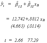
Using a t-test we can seehas a significant impact on y.

We could also do the test using ANOVA

So again, the model is significant.

Now let us add the time trend and see if it adds significantly to the explanation of y.

In order to do this we construct a new ANOVA table

Source	SS	df
ESS due to x2 alone		1
ESS due to addition of x3		1
ESS due to x2 and x3		2
RSS		n-3
TSS		n-1

To assess the contribution ofafter allowing forwe form the F statistic

for our example

which is significant.

The advantage to ANOVA is that we can do sets of variables while controlling for sets already included.